
Note: This is an automated translation (using DeepL) of the original German article.
The dynamics of omicron wave and quarantine cases depend heavily on the spread of subvariant BA.2. But how does this work?
The dynamics of the Covid-19 pandemic are constantly changing. This is and has been most obvious in the “peaks” in case numbers. Currently, however, a change is taking place that is only partially visible from the outside: the change in dominance from BA.1 to BA.2.
The effects of this change are illustrated in Figure 1, which shows three theoretical forecast scenarios for Upper Austria that differ from each other “only” by the BA.2 start rate (“start prevalence”). The collected data for BA.2 prevalence are samples, which are subject to fluctuations depending on the source and sample size. To cover this range of variation for the data from calendar week 5 (Jan. 31-Feb. 6, 2022), scenarios of 4% and 12% were calculated in addition to the likely mean of 8% BA.2 prevalence.
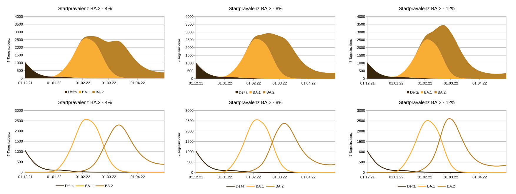
Figure 1: It can be seen how the peak of the BA.2 wave with higher start prevalence not only occurs earlier, but also turns out higher. From left to right: scenario with slightly reduced BA.2 starting level, baseline scenario with BA.2 level according to real data estimate, scenario with slightly increased BA.2 starting prevalence. Due to the age of the content it is to be understood as example and not as current model (graphic in full resolution).
In the figure below, the curves for variants Delta, Omicron-BA.1 and Omicron-BA.2 are shown separately. The graphs in the upper row show the sums of the individual curves. In the simulation, it can be seen that faster dominance adoption of BA.2 results in earlier and higher BA.2 curves (lower graphs). This in turn leads (upper graphs) to a steeper overall epidemic curve.
In turn, a steeper epidemic curve means that, under current rules, more people have to be in quarantine simultaneously - which in turn has a direct impact on social life (school closures, supplies and infrastructure, …). Therefore, in order to reduce the number of people in quarantine at the same time, it makes sense to flatten the curve in its height.
Relaxations in the rise of the curve reinforce the dynamics. In contrast, relaxations after a peak has been crossed have a much smaller impact in relative terms. This is partly due to the fact that the measured dynamics lags the real dynamics by about a week, i.e. when the peak occurs in the measurements, the real dynamics already goes down rapidly.
Overall, it is therefore recommended that the dynamics of BA.1 and BA.2 be considered separately and that relaxations (subject to no new virus variants) be made dependent on the peak time of the BA.2 variant. Whether and for how long the numbers of positive tests will continue to be relevant is a social and political discussion that absolutely must be held.
Overlapping waves
To illustrate the impact of two overlapping epidemic waves, an example scenario was calculated using a highly simplified model. Here, the start of propagation of the BA.2 wave is pushed back in each simulation run. Figure 2 shows the resulting epidemic curves and their overlap. Also marked (with a vertical black line) is the time at which the BA.2 variant accounts for one percent of all infections.
Figure 2: Effect of timing of first emergence (1% of new daily infections) of BA.2 variant on observed case incidence.
The animation shows the effect of the timing of the BA.2 peak. If it coincides with the BA.1 peak (on the left of the figure), the result is a high overall peak. If the BA.2 peak moves further back, first the curve flattens. If the second peak is far enough away from the first, the two waves separate and become recognizable as separate waves.