Didactic Pendulum Simulation
In the course of a longstanding series of lectures at Vienna University of Technology different technical approaches in teaching assistance were developed. Besides interactive online tools for presenting applied examples in mathematics and modeling/simulation, also hands-on experiments designed for lectures and events were developed in cooperation of TU Vienna and dwh simulation services.
The following setup of a classical pendulum serves the illustration of basic concepts of modeling and simulation:
- system abstraction and model simplification
- physical modeling with ordinary differential equations
- implementation of realtime simulation (ODE-solver) and visualization
- validation of simulation models
Assembly and Structure of the Experiment
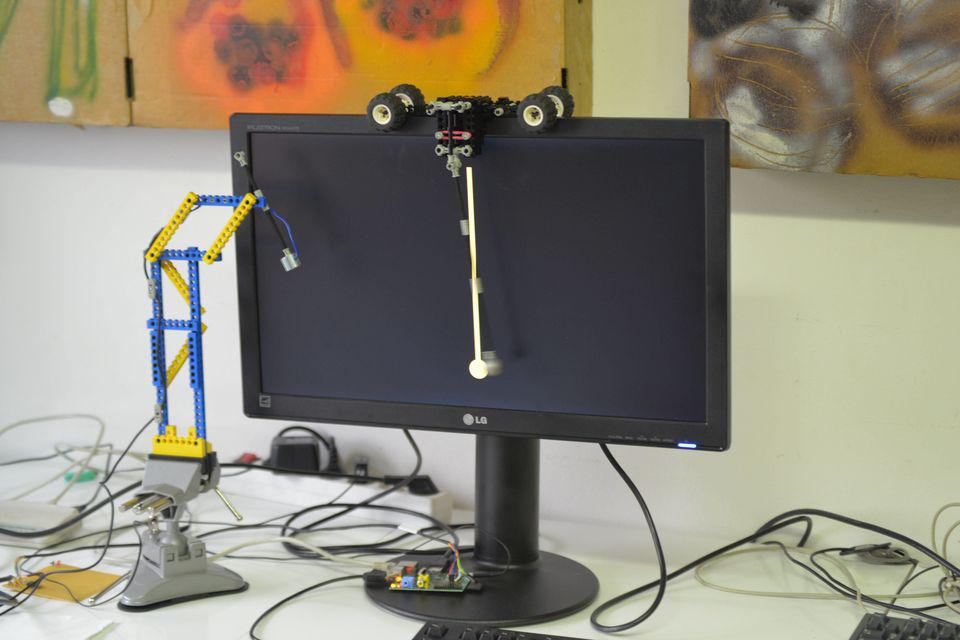
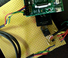
A pendulum with metal ball is placed in front of a computer monitor. An electromagnetic device at the side can keep the pendulum in its initial position and release it in a controlled manner. The electromagnet is controlled via a Raspberry Pi minicomputer which also runs the simulation program. The simulation is started synchronously to releasing the pendulum by turning off the magnet and to starting a realtime visual animation of the simulated pendulum on the screen.
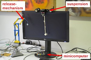
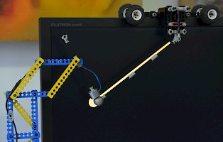
Assembly with Lego components. The suspension of the pendulum is mounted on the monitor bezel.
By adjusting the position of the electromagnetic release device, arbitrary initial conditions (displacement of the pendulum) can be chosen. Via keyboard entry, the initial displacement of the virtual pendulum can be adjusted to the pendulum in front of the screen.
With another keyboard entry the experiment is started. The electromagnet is turned off and simulation as well as visual output commence.
After a certain amount of time differences arise between the pendulum and its simulated counterpart. The differences are caused by multiple factors and are part of the presentation of the experiment.
Via configuration files and a configuration menu it is possible to adjust the parameters of the model. Hence the pendulum can be simulated with different parameters or parameter sets which can be predefined or modified in an interactive way. The configuration files must be adapted to fit the dimensions of the pendulum (masses, lengths, friction coefficients).
Technical Implementation
Hardware
The assembly requires basic knowledge about electricity and soldering of circuits. The following or similar electronic components are required:
Warning: Improper handling with electricity can be dangerous!
- Raspberry Pi 1 B
- 32-bit ARMv6 Single Core 700 MHz CPU
- OpenGL-ES 2.0 compatible GPU
- Circuit
- Transistor (TIP122)
- Resistor 1kOhm
- Diode (1n4007) 1kV 1A
- Electromagnet specified for 12V
- Power Supply
- 5V 1.5A and 12V 1.5A
The Raspberry Pi minicomputer is equipped with GPIO ports (see documentation) which can be used for controlling the electromagnet. Additionally the minicomputer can be powered via GPIO ports instead of micro-USB.
Warning: Improper use of the ports can damage the device (see documentation)!
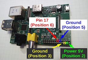
A possible configuration of GPIO ports on the Raspberry Pi 1 B for connecting the circuit (see below) and for power supply.
Via a transistor the power supply of the electromagnet is controlled. The transistor can be switched with a signal from the GPIO ports of the minicomputer. Power supplies and signal connection can be implemented in a single circuit .
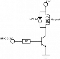
Schematic circuit (without power supply of the minicomputer).
Software
The control and simulation program is written in C. The code is available under the GPLv3 license. Following libraries are required:
| Library | Links | Description |
|---|---|---|
| libxml2 | configuration files | |
| ncurses, cdk | configuration menu | |
| OpenGL ES, EGL | Raspberry Pi VideoCore APIs | visualization |
| GSL | GSL – Ordinary Differential Equations | ODE-solver |
At startup the program is in configuration mode. Positioning, lengths and initial angle of displacement can be adjusted and saved via keyboard entry.
After triggering the simulation (and concurrent release of the magnet) alternating the pendulum equation is solved up to a precalculated time point and the displacement of the pendulum is drawn on the screen (realtime simulation).
When the simulation is canceled the program returns to its configuration mode.